Imitation learning

---

source

PS_imitation

 PS_imitation (num_states:int, eta:float, gamma:float)

Constructs a PS agent with two actions (continue and rotate) that performs imitation learning in the search scenario. Instead of following a full trajectory of action-state tuples, the agent is directly given the reward state (the step length in this case). The agent updates all previous continue actions and the current rotate action.

	Type	Details
num_states	int	Number of states
eta	float	Glow parameter of PS
gamma	float	Damping parameter of PS

---

source

PS_imitation.update

 PS_imitation.update (length:int, reward:int=1)

Updates the policy based on the imitation scheme (see paper for detailes)
NOTE: state is length-1 because counter starts in 0 (but in 0, agent has already performed a step of length 1 – from the previous action “rotate”).

	Type	Default	Details
length	int		Step length rewarded
reward	int	1	Value of the reward

Example

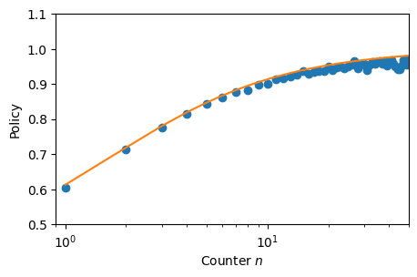
We showcase how to imitate the policy based on a given step length distribution, an in particular of a Lévy distribution. For further examples, see the Tutorials section.

from rl_opts.analytics import pdf_powerlaw, pdf_discrete_sample, get_policy_from_dist
from tqdm import tqdm
import matplotlib.pyplot as plt
import numpy as np

NUM_STATES = 100 # size of the state space
EPOCHS = 100 # number of epochs
NUM_STEPS = 1000 # number of learning steps per episode

steps = pdf_discrete_sample(pdf_func = pdf_powerlaw,
                            beta = 1,
                            L = np.arange(1, NUM_STATES),  
                            num_samples = (EPOCHS, NUM_STEPS))

imitator = PS_imitation(num_states = NUM_STATES,
                        eta = int(1e-7),
                        gamma = 0)
    
                               
for e in tqdm(range(EPOCHS)):
    imitator.reset()
    for s in steps[e]:    
        imitator.update(length = s)

100%|██████████| 100/100 [00:01<00:00, 86.11it/s]

policy_theory = get_policy_from_dist(n_max = NUM_STATES,
                                     func = pdf_powerlaw,
                                     beta = 1)
policy_imitat = imitator.h_matrix[0,:]/imitator.h_matrix.sum(0)

_ , ax = plt.subplots(figsize = (5,3))
ax.plot(policy_imitat ,'o')
ax.plot(np.arange(1, NUM_STATES), policy_theory[1:])
plt.setp(ax, 
         xscale = 'log', xlim = (0.9, NUM_STATES/2), xlabel = r'Counter $n$',
         ylim = (0.5, 1.1), ylabel = 'Policy');